How to Calculate Q1 and Q3: The Definitive Statistical Guide for Data Analysis
The first and third quartiles—Q1 and Q3—are the unsung heroes of statistical analysis. While means and medians dominate headlines, these quartiles quietly reveal the hidden structure of datasets, exposing dispersion, skewness, and outliers with surgical precision. Without them, box plots would be hollow shells, and trend analysis would lack depth. Yet, many professionals either misapply them or overlook their nuanced role in decision-making.
Calculating Q1 and Q3 isn’t just a mechanical exercise; it’s a gateway to understanding how data behaves beyond averages. Whether you’re analyzing market trends, assessing performance metrics, or debugging algorithms, these quartiles provide the granularity missing from surface-level summaries. The difference between a superficial glance at data and a strategic, informed interpretation often hinges on whether you’ve correctly identified Q1 and Q3.
Missteps here can lead to flawed conclusions—imagine a financial analyst misjudging risk because quartiles were mishandled, or a quality control team overlooking critical deviations. The stakes are higher than most realize. This guide cuts through the ambiguity, offering a rigorous, step-by-step breakdown of how to calculate Q1 and Q3 with clarity, precision, and practical relevance.

The Complete Overview of Understanding Quartiles
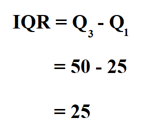
Quartiles divide a dataset into four equal parts, each representing 25% of the data. Q1 (the first quartile) marks the 25th percentile, while Q3 (the third quartile) sits at the 75th percentile. Together, they form the backbone of the interquartile range (IQR), a measure of statistical dispersion that’s far more robust than standard deviation in skewed distributions. Unlike percentiles, which can be arbitrary, quartiles provide a fixed framework for comparing data segments.
The significance of Q1 and Q3 extends beyond academia. In business, they help identify performance quartiles—top 25% vs. bottom 25%—for resource allocation. In healthcare, they reveal patient response variability to treatments. Even in machine learning, quartiles are used to detect anomalies in training datasets. Yet, their calculation isn’t universal; methods vary by field, and errors in interpolation or dataset ordering can distort results. Understanding how to calculate Q1 and Q3 accurately is non-negotiable for credible analysis.
Historical Background and Evolution
The concept of quartiles emerged in the late 19th century as statisticians sought to standardize ways of summarizing large datasets. Early methods were ad-hoc, relying on manual sorting and division. The 1920s saw the rise of formalized quartile definitions, particularly in agricultural and economic studies, where data variability was critical. By the mid-20th century, quartiles became integral to exploratory data analysis (EDA), thanks to John Tukey’s influence, who popularized the box plot—a visual tool that hinges on Q1 and Q3.
Table of Contents
- The Complete Overview of Understanding Quartiles
- Historical Background and Evolution
- Core Mechanisms: How It Works
- Key Benefits and Crucial Impact
- Major Advantages
- Comparative Analysis
- Future Trends and Innovations
- Conclusion
- Comprehensive FAQs
- Q: What’s the difference between quartiles and percentiles?
- Q: Can Q1 and Q3 be the same in a dataset?
- Q: Why does Excel’s QUARTILE function sometimes give different results than manual calculations?
- Q: How do quartiles help in identifying outliers?
- Q: Are there industry-specific standards for calculating quartiles?
Modern computing has democratized quartile calculations, but the underlying principles remain rooted in statistical theory. Today, software like Python, R, and Excel automate the process, yet manual calculation techniques persist in educational settings and domains requiring transparency (e.g., auditing). The evolution of how to calculate Q1 and Q3 reflects broader trends in data science: from manual labor to algorithmic efficiency, while preserving the core logic of dividing data into meaningful quartiles.
Core Mechanisms: How It Works
At its core, calculating Q1 and Q3 involves two steps: sorting the data and applying a position formula. The dataset must first be ordered from least to greatest. The position of Q1 is determined by the formula P = (n + 1) × (p/100), where n is the number of data points and p is the percentile (25 for Q1, 75 for Q3). If P is an integer, the quartile is the average of the values at positions P and P-1. If P is not an integer, interpolation is used to estimate the quartile.
For example, in a dataset of 10 values, Q1’s position would be (10 + 1) × 0.25 = 2.75. This means Q1 is the 25th percentile, calculated by interpolating between the 2nd and 3rd values. The choice of interpolation method (linear, nearest rank, etc.) can yield slightly different results, which is why standards like the Tukey’s hinges method exist. Mastering these mechanics ensures consistency when answering how to calculate Q1 and Q3 in practice.
Key Benefits and Crucial Impact
Quartiles are more than just statistical curiosities—they are tools for uncovering patterns that means and standard deviations obscure. By focusing on the middle 50% of data (Q1 to Q3), analysts can identify trends in central tendency without being skewed by extreme values. This is particularly valuable in fields like finance, where outliers (e.g., market crashes) can distort averages. Quartiles also enable robust benchmarking: comparing Q1 and Q3 across datasets reveals relative performance without the noise of extreme data points.
The interquartile range (IQR), derived from Q1 and Q3, is a cornerstone of outlier detection. Any data point beyond Q3 + 1.5 × IQR or below Q1 - 1.5 × IQR is flagged as an outlier—a critical feature in quality control, fraud detection, and anomaly monitoring. Without Q1 and Q3, these systems would lack precision. Understanding how to calculate Q1 and Q3 correctly is thus essential for building reliable analytical frameworks.
"Quartiles are the silent architects of data integrity. They don’t just describe—they reveal the story behind the numbers."
— Dr. Harold W. Dodge, Statistician and Data Visualization Pioneer
Major Advantages
- Robustness to Outliers: Unlike mean-based metrics, quartiles are resistant to extreme values, making them ideal for skewed distributions.
- Precision in Benchmarking: Q1 and Q3 provide clear thresholds for comparing performance across groups (e.g., top 25% vs. bottom 25%).
- Foundation for Box Plots: Box plots, a staple in exploratory data analysis, rely entirely on Q1, Q3, and the median.
- Regulatory Compliance: Industries like finance and healthcare use quartiles for risk assessment and quality standards.
- Algorithm Optimization: In machine learning, quartiles help balance datasets and detect training anomalies.

Comparative Analysis
| Method | Description |
|---|---|
| Linear Interpolation | Most common; estimates quartiles by averaging adjacent values. Used in Excel’s QUARTILE function. |
| Nearest Rank Method | Rounds the position to the nearest integer, then selects the corresponding value. Simpler but less precise. |
| Tukey’s Hinges | Uses a weighted average for positions, favored in robust statistics. Less sensitive to small dataset fluctuations. |
| Mood’s Median Method | Recursively applies median calculations to halves of the data. Rarely used but theoretically sound. |
Future Trends and Innovations
The future of quartile calculations lies in automation and adaptive methods. As datasets grow exponentially, traditional interpolation techniques may struggle with scalability. Machine learning models are now being trained to predict quartiles dynamically, adjusting for data density and distribution. Additionally, real-time quartile analysis—critical in IoT and financial trading—is pushing for low-latency algorithms that can process streaming data without batch delays.
Another frontier is the integration of quartiles with big data frameworks like Apache Spark. These systems optimize quartile computation across distributed datasets, enabling enterprises to analyze terabytes of data without manual intervention. For professionals, staying ahead means embracing these innovations while retaining the fundamental principles of how to calculate Q1 and Q3 accurately in both traditional and emerging contexts.
Conclusion
Quartiles are not just statistical footnotes—they are the lens through which data’s true character emerges. Whether you’re a data scientist, a business analyst, or a student of statistics, the ability to calculate Q1 and Q3 with confidence is a skill that elevates analysis from basic reporting to strategic insight. The methods outlined here—from manual interpolation to software-driven automation—ensure that you can apply quartiles correctly, regardless of the dataset or tool.
As data continues to reshape industries, the demand for precise, quartile-based analysis will only grow. By mastering how to calculate Q1 and Q3, you’re not just learning a technique; you’re equipping yourself with a tool to navigate complexity, detect anomalies, and make decisions grounded in data—not assumptions.
Comprehensive FAQs
Q: What’s the difference between quartiles and percentiles?
A: Quartiles divide data into four equal parts (25th, 50th, 75th percentiles), while percentiles can represent any division (e.g., 10th, 90th). Quartiles are a subset of percentiles, specifically the 25th (Q1) and 75th (Q3) percentiles.
Q: Can Q1 and Q3 be the same in a dataset?
A: Yes, in a perfectly uniform dataset (all values identical), Q1 and Q3 will coincide with the median. However, this is rare in real-world data.
Q: Why does Excel’s QUARTILE function sometimes give different results than manual calculations?
A: Excel uses linear interpolation by default (Method 2 in older versions), while manual methods may employ Tukey’s hinges or nearest rank. Always specify the method for consistency.
Q: How do quartiles help in identifying outliers?
A: The IQR (Q3 - Q1) defines a range. Values beyond Q3 + 1.5 × IQR or below Q1 - 1.5 × IQR are flagged as outliers, a technique known as the 1.5×IQR rule.
Q: Are there industry-specific standards for calculating quartiles?
A: Yes. Finance uses modified quartiles for risk metrics (e.g., Value-at-Risk), while healthcare may apply weighted quartiles for patient response studies. Always align with domain-specific guidelines.
Leave a Comment
Comments are moderated before appearing. The data you submit is processed according to the Privacy Policy of Bevvy.