How Do You Find the Interquartile Range? The Definitive Statistical Method
Understanding how do you find the interquartile range (IQR) is a cornerstone of statistical analysis, yet it remains one of the most misunderstood concepts for both students and professionals. The IQR isn’t just a number—it’s a window into data distribution, revealing where the bulk of values lie while filtering out extreme outliers. Unlike standard deviation, which measures spread around the mean, the IQR focuses on the middle 50% of data, making it far more resilient to skewed distributions or anomalous values. This resilience is why financial analysts, healthcare researchers, and quality control engineers rely on it to assess variability without distortion.
The process of how to calculate the interquartile range seems straightforward at first glance: identify the first (Q1) and third (Q3) quartiles, then subtract Q1 from Q3. But the devil lies in the details. Should you use the nearest-rank method, linear interpolation, or Tukey’s hinges? Each approach yields slightly different results, especially with small datasets or unevenly distributed values. These nuances explain why even seasoned statisticians debate the "correct" way to find the interquartile range—a debate that hinges on the intended use case, from exploratory data analysis to hypothesis testing.
What makes the IQR uniquely powerful is its role in visualizing data through box plots, where it defines the "box" that encapsulates the central tendency. It’s also the foundation for detecting outliers using the 1.5×IQR rule, a technique employed in fields ranging from manufacturing defect analysis to sports performance metrics. Yet, despite its ubiquity, many practitioners overlook its full potential, treating it as a mere checkbox in statistical reports. This guide dismantles that limitation, offering a rigorous breakdown of how to find the interquartile range—from foundational principles to real-world applications—while addressing common pitfalls that distort results.
###

The Complete Overview of How to Find the Interquartile Range
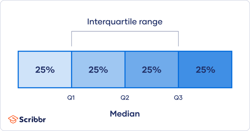
The interquartile range (IQR) is a measure of statistical dispersion that quantifies the spread of the middle 50% of a dataset. Unlike range (which captures the distance between the minimum and maximum values), the IQR isolates variability within the interquartile span, making it less sensitive to outliers. This distinction is critical in fields like epidemiology, where extreme values (e.g., a single patient’s unusually high cholesterol reading) can skew interpretations if not properly accounted for. The IQR’s robustness stems from its focus on quartiles—values that divide the data into four equal parts—allowing analysts to find the interquartile range by simply measuring the distance between Q1 (the 25th percentile) and Q3 (the 75th percentile).However, the simplicity of the concept belies the complexity of its calculation. The method for how to calculate the interquartile range varies depending on the dataset’s size and the statistical convention used. For example, with 10 data points, Q1 might be the average of the 2nd and 3rd values, while Q3 could be the average of the 8th and 9th. But with 11 points, the quartiles might align with the 3rd and 9th values directly. These discrepancies arise because quartiles are not fixed positions but depend on whether the dataset’s size is odd or even, and whether the calculation method favors interpolation or discrete ranking. This variability is why understanding how do you find the interquartile range requires more than memorization—it demands an appreciation for the underlying methodology’s flexibility.
###
Historical Background and Evolution
The origins of quartiles and the interquartile range trace back to the 18th century, when statisticians sought ways to summarize large datasets without relying solely on measures like the mean or median. Early pioneers, including Carl Friedrich Gauss and Francis Galton, recognized that central tendency metrics alone couldn’t capture the full picture of data distribution. The concept of dividing data into quartiles emerged as a practical solution, particularly in agricultural and biological studies where variability was a key concern. By the early 20th century, statisticians like George W. Snedecor formalized the IQR as a tool for assessing dispersion, distinguishing it from the more volatile range.Table of Contents
- The Complete Overview of How to Find the Interquartile Range
- Historical Background and Evolution
- Core Mechanisms: How It Works
- Key Benefits and Crucial Impact
- Major Advantages
- Comparative Analysis
- Future Trends and Innovations
- Conclusion
- Comprehensive FAQs
- Q: What’s the difference between the interquartile range and standard deviation?
- Q: Can I use the IQR to compare two datasets?
- Q: Why does the method for finding the interquartile range matter?
- Q: How does the IQR relate to box plots?
- Q: Is the IQR always better than the range for measuring spread?
- Q: Can I calculate the IQR for categorical data?
- Q: How does sample size affect the IQR calculation?
- Q: What’s the 1.5×IQR rule for outliers?
- Q: Can the IQR be negative?
- Q: How do I find the IQR in Python?
The evolution of how to find the interquartile range reflects broader shifts in statistical thinking. Initially, quartiles were calculated using simple percentile methods, but as computing power advanced, more sophisticated techniques—such as linear interpolation—gained traction. Today, the debate over the "best" method persists, with proponents of Tukey’s hinges (used in box plots) arguing for a more robust approach to handling small datasets. This historical context underscores why the IQR isn’t a static concept but one that adapts to the needs of modern data analysis, from machine learning to climate science.
###
Core Mechanisms: How It Works
At its core, how to calculate the interquartile range involves three steps: ordering the data, locating Q1 and Q3, and computing their difference. The first step is straightforward—sorting the dataset in ascending order—but the second introduces complexity. For instance, in a dataset of 20 values, Q1 would be the median of the first 10 values, while Q3 would be the median of the last 10. However, if the dataset has 21 values, Q1 might be the 6th value (using the "nearest-rank" method), or the average of the 5th and 6th values (using interpolation). This ambiguity is why textbooks often present multiple methods for how do you find the interquartile range, each with trade-offs in precision and computational simplicity.The choice of method also affects how outliers are identified. The 1.5×IQR rule, for example, defines outliers as values below Q1 – 1.5×IQR or above Q3 + 1.5×IQR. But if Q1 and Q3 are calculated differently, the outlier thresholds shift accordingly. This sensitivity is why data scientists must align their method for how to find the interquartile range with the analysis’s goals—whether detecting anomalies in cybersecurity logs or assessing variability in experimental results.
###
Key Benefits and Crucial Impact
The interquartile range’s strength lies in its ability to provide a clear, outlier-resistant measure of spread. Unlike standard deviation, which can be inflated by extreme values, the IQR remains stable even in skewed distributions. This property makes it indispensable in fields where data quality is uncertain, such as survey research or sensor measurements. For example, a market researcher analyzing consumer income might use the IQR to describe the typical range without being misled by a few high-earning outliers. Similarly, in quality control, manufacturers rely on the IQR to monitor production consistency, where even minor shifts in variability can signal process drift.Beyond its practical utility, the IQR serves as a gateway to deeper statistical insights. It’s a key component in the five-number summary (minimum, Q1, median, Q3, maximum), which underpins box plots—a visualization tool that reveals skewness, symmetry, and outliers at a glance. This visual clarity is why the IQR is taught alongside exploratory data analysis (EDA) techniques, bridging the gap between raw numbers and actionable conclusions.
> "The interquartile range is not just a measure of spread; it’s a lens through which we can see the true structure of data, unobscured by the noise of extremes." > — John Tukey, Statistician and Pioneer of Exploratory Data Analysis
###
Major Advantages
- Robustness to Outliers: Unlike range or standard deviation, the IQR is unaffected by extreme values, making it ideal for datasets with skewed distributions or measurement errors.
- Simplicity in Interpretation: The IQR directly answers the question, "What’s the typical spread of the middle 50% of data?"—a more intuitive metric than variance or standard deviation.
- Foundation for Outlier Detection: The 1.5×IQR rule provides a data-driven threshold for identifying anomalies, critical in fields like fraud detection or manufacturing defect analysis.
- Compatibility with Box Plots: As the "box" in a box plot, the IQR visually communicates central tendency and variability, aiding in quick data diagnostics.
- Non-Parametric Nature: The IQR doesn’t assume a normal distribution, making it versatile for non-normal or small datasets where parametric methods fail.

Comparative Analysis
| Metric | Interquartile Range (IQR) |
|---|---|
| Definition | Distance between Q1 (25th percentile) and Q3 (75th percentile). |
| Sensitivity to Outliers | Low (ignores extreme values). |
| Use Case | Exploratory data analysis, box plots, outlier detection. |
| Calculation Dependency | Dataset size and quartile method (e.g., nearest-rank vs. interpolation). |
Future Trends and Innovations
As data science evolves, the IQR’s role is expanding beyond traditional statistics. In machine learning, quartile-based feature scaling (e.g., robust scaling) is gaining popularity to handle skewed or high-dimensional data. Meanwhile, in big data analytics, approximate quartile algorithms are being developed to compute the IQR efficiently on massive datasets without full sorting. These innovations reflect a broader trend: leveraging the IQR’s simplicity and robustness to solve problems where classical methods fall short.Another frontier is the integration of the IQR with probabilistic programming frameworks, where Bayesian statisticians use quartiles to model uncertainty in predictive models. As datasets grow more complex—incorporating time-series, categorical, and multimodal data—the IQR’s adaptability will be tested. Yet, its core principle—focusing on the middle 50%—remains timeless, ensuring that how to find the interquartile range will continue to be a fundamental skill for data-driven decision-making.
###
Conclusion
The interquartile range is more than a statistical formula; it’s a tool for uncovering the hidden patterns in data. Whether you’re a student learning how to calculate the interquartile range for the first time or a data scientist refining outlier detection models, mastering this concept unlocks a deeper understanding of variability. The key lies in recognizing that the "correct" method for how do you find the interquartile range depends on the context—whether prioritizing computational speed, visual clarity, or robustness to outliers.As data grows in volume and complexity, the IQR’s relevance only increases. It bridges the gap between raw numbers and meaningful insights, serving as both a diagnostic tool and a foundation for more advanced analyses. For those who ask, "How do you find the interquartile range?"—the answer isn’t just a calculation, but a mindset: one that values the middle ground over the extremes.
###
Comprehensive FAQs
Q: What’s the difference between the interquartile range and standard deviation?
The IQR measures the spread of the middle 50% of data and is robust to outliers, while standard deviation measures average deviation from the mean and is sensitive to extreme values. Use the IQR for skewed data or outlier-prone datasets.
Q: Can I use the IQR to compare two datasets?
Yes, but only if the datasets are on the same scale and have similar distributions. A larger IQR indicates greater variability in the middle 50% of data, making it useful for relative comparisons.
Q: Why does the method for finding the interquartile range matter?
Different methods (e.g., nearest-rank vs. interpolation) yield slightly different Q1 and Q3 values, which can affect outlier thresholds and box plot representations. Consistency within a project is key.
Q: How does the IQR relate to box plots?
The IQR defines the "box" in a box plot, with Q1 and Q3 marking its edges. Whiskers extend to 1.5×IQR beyond Q1/Q3, and dots beyond that indicate outliers.
Q: Is the IQR always better than the range for measuring spread?
Not necessarily. The range is simpler and useful for symmetric, outlier-free data, while the IQR excels in skewed or noisy datasets. Choose based on data characteristics.
Q: Can I calculate the IQR for categorical data?
No. The IQR requires numerical, ordered data. For categorical variables, use frequency distributions or chi-square tests instead.
Q: How does sample size affect the IQR calculation?
Smaller datasets may produce less stable quartiles, especially with discrete methods. Interpolation methods (e.g., linear) are often preferred for n < 50 to reduce variability.
Q: What’s the 1.5×IQR rule for outliers?
Values below Q1 – 1.5×IQR or above Q3 + 1.5×IQR are flagged as outliers. This rule balances sensitivity and specificity for most applications.
Q: Can the IQR be negative?
No. Since Q3 ≥ Q1 by definition, the IQR is always non-negative. A negative result suggests an error in quartile calculation.
Q: How do I find the IQR in Python?
Use `pandas` or `numpy`:
For box plots, use `matplotlib` or `seaborn`.import numpy as np
data = np.array([...])
q1, q3 = np.percentile(data, [25, 75])
iqr = q3 - q1
Leave a Comment
Comments are moderated before appearing. The data you submit is processed according to the Privacy Policy of Bevvy.