How the pandas dataframe revolutionized data science
The pandas dataframe isn’t just another Python data structure—it’s the quiet architect behind some of the most influential data-driven decisions in finance, healthcare, and AI. Built on decades of numerical computing evolution, it bridges the gap between raw tabular data and actionable insights, handling everything from messy CSV imports to complex multi-index hierarchies with surgical precision. What makes it truly indispensable isn’t its speed (though it’s optimized for performance), but its ability to feel intuitive—like a spreadsheet that understands Python’s syntax while preserving the flexibility of SQL queries.
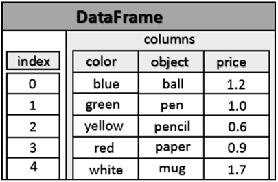
At its core, the pandas dataframe represents a two-dimensional, size-mutable, and heterogeneous tabular data structure. Unlike traditional arrays or dictionaries, it enforces a columnar structure where each column can hold different data types—integers, strings, dates, or even nested objects—while maintaining alignment across rows. This design mirrors how real-world data is often structured: relational, hierarchical, and frequently inconsistent. The genius lies in its balance: it’s rigorous enough for statistical analysis yet adaptable enough to handle the chaos of production datasets.
The first time you reshape a messy dataset into a clean dataframe with a single command—filtering outliers, pivoting dimensions, or merging tables—you understand why teams across industries have adopted it as their default tool. It’s not just about efficiency; it’s about clarity. When a financial analyst needs to merge quarterly reports with customer transaction logs, or a biostatistician must align clinical trial data with genomic sequences, the pandas dataframe becomes the invisible thread holding the analysis together.

The Complete Overview of pandas dataframe
The pandas dataframe is the linchpin of Python’s data science ecosystem, serving as both a container and a processing engine for structured data. Its origins trace back to the need for a tool that could handle the growing complexity of datasets in the 2000s, when traditional statistical packages like R and MATLAB struggled to scale with modern computational demands. What began as a personal project by Wes McKinney in 2008—inspired by R’s data.frame but designed for Python’s flexibility—quickly became the de facto standard for data manipulation. By 2010, its integration into the open-source community transformed it from a niche utility into a cornerstone of data workflows, powering everything from exploratory analysis to large-scale machine learning pipelines.Today, the pandas dataframe isn’t just a library feature; it’s a cultural artifact of how data is processed. Its adoption reflects a broader shift in the field: away from rigid, domain-specific tools and toward general-purpose frameworks that can adapt to diverse use cases. Whether you’re cleaning a dataset for a Kaggle competition or building a real-time analytics dashboard, the pandas dataframe provides the foundational operations—filtering, grouping, merging, and transforming—that turn raw data into meaningful patterns. Its ubiquity stems from solving a fundamental problem: how to make tabular data programmable without sacrificing readability.
Historical Background and Evolution
The development of pandas was a direct response to the limitations of Python’s existing numerical computing tools in the late 2000s. Before pandas, data scientists relied on a patchwork of solutions: NumPy for arrays, dictionaries for heterogeneous data, and custom scripts for operations like pivoting or time-series alignment. Wes McKinney, a quant at AQR Capital Management, recognized that these approaches were inefficient and error-prone, especially when dealing with financial datasets that required frequent reshaping and aggregation. His goal was to create a library that combined the ease of R’s data.frame with Python’s extensibility, while adding features like built-in handling of missing data and time-series functionality.The first public release of pandas in 2009 was met with immediate acclaim, particularly in the quantitative finance community. By 2012, its inclusion in the SciPy stack solidified its role as a foundational tool, and the introduction of the `merge()` and `groupby()` operations further cemented its dominance. Key milestones—such as the addition of multi-indexing in version 0.13 (2014) and the optimization of C-based backends—demonstrated a commitment to performance without sacrificing usability. Today, pandas is maintained by a global team of contributors, with major releases introducing features like nullable integer dtypes, query compilation, and integration with Apache Arrow, ensuring it remains at the forefront of data manipulation.
Core Mechanisms: How It Works
Under the hood, the pandas dataframe is built on three interconnected layers: the data model, the indexing system, and the optimized operations. The data model leverages NumPy arrays for homogeneous data (e.g., numeric columns) and Python objects for heterogeneous data (e.g., mixed types in a single column), with a metadata layer tracking column names, dtypes, and memory layout. This hybrid approach allows it to balance speed and flexibility—critical for datasets ranging from small CSV files to multi-gigabyte tables.Table of Contents
- The Complete Overview of pandas dataframe
- Historical Background and Evolution
- Core Mechanisms: How It Works
- Key Benefits and Crucial Impact
- Major Advantages
- Comparative Analysis
- Future Trends and Innovations
- Conclusion
- Comprehensive FAQs
- Q: How does the pandas dataframe handle missing data?
- Q: Can the pandas dataframe work with databases directly?
- Q: What’s the difference between `df.loc` and `df.iloc`?
- Q: How does the pandas dataframe optimize memory usage?
- Q: Is the pandas dataframe thread-safe for concurrent operations?
- Q: How can I improve performance for large datasets?
The indexing system is where pandas shines. Unlike traditional arrays, which rely on positional indices, pandas uses labels (via `Index` objects) to identify rows and columns, enabling operations like partial string matching (`df.loc['2023-01']`) or hierarchical indexing (MultiIndex). This label-based approach mirrors how humans interact with data—by meaning rather than position—and underpins features like `groupby()`, which partitions data by arbitrary keys. Underlying these operations is a vectorized engine that avoids Python loops by delegating work to optimized C/Fortran routines, ensuring that even complex transformations (e.g., `df.apply()`) execute efficiently.
Key Benefits and Crucial Impact
The pandas dataframe’s influence extends beyond its technical capabilities—it has redefined how data teams approach problems. In industries where data is the primary asset, the ability to quickly prototype, validate, and iterate on analyses translates to competitive advantages. Financial institutions use it to backtest trading strategies; healthcare researchers rely on it to correlate patient data with treatment outcomes; and tech companies deploy it to analyze user behavior at scale. The tool’s impact isn’t just in speed but in democratization: it lowers the barrier for non-programmers to perform advanced analytics, while giving experts the precision they need.At its heart, the pandas dataframe solves three critical challenges: data integration, analysis agility, and reproducibility. It seamlessly merges datasets from disparate sources (SQL, Excel, APIs), applies transformations without manual coding, and preserves metadata (column names, data types) to ensure analyses remain interpretable. This combination of power and accessibility has made it the default choice for data scientists, analysts, and engineers alike.
"Pandas didn’t just improve data analysis—it made it feel like a conversation between the data and the analyst. Before pandas, you were fighting the tool; now, the tool fights for you." — Hadley Wickham, Chief Scientist at RStudio
Major Advantages
- Unified Data Handling: Supports mixed data types (e.g., strings, dates, and numeric values) in a single structure, eliminating the need for separate containers like dictionaries or lists.
- Performance Optimizations: Leverages NumPy’s vectorized operations and lazy evaluation (via `query()`) to execute transformations at near-C speeds, even on large datasets.
- Rich Ecosystem: Integrates seamlessly with libraries like Matplotlib (visualization), scikit-learn (ML), and Dask (parallel computing), forming the backbone of Python’s data stack.
- Time-Series Ready: Built-in support for datetime indexing and resampling (e.g., `df.resample('M')`) simplifies financial and scientific time-series analysis.
- Memory Efficiency: Uses sparse matrices and downcasting (e.g., `pd.to_numeric(downcast='integer')`) to reduce memory footprint without sacrificing functionality.
Comparative Analysis
| Feature | pandas dataframe | R data.frame | SQL Tables |
|---|---|---|---|
| Data Type Flexibility | Mixed types per column (e.g., strings + numbers) | Homogeneous columns (all elements same type) | Strict schema enforcement (fixed dtypes per column) |
| Indexing | Label-based (MultiIndex, datetime) | Positional + named indices | Primary keys only (no hierarchical labels) |
| Performance | Optimized C backend, vectorized ops | Slower for large datasets (interpreted) | Fast for queries, slow for transformations |
| Learning Curve | Moderate (Python syntax familiarity helps) | Steep (R’s functional paradigm) | High (SQL query complexity) |
Future Trends and Innovations
The next evolution of the pandas dataframe will likely focus on scalability and interoperability. As datasets grow beyond memory limits, projects like Dask and Modin are extending pandas’ functionality to distributed computing, while Apache Arrow’s adoption as a memory format promises faster data exchange between languages (Python, R, Java). Another frontier is automated data cleaning: tools like Pandas-Profiling and AutoViz are already integrating with pandas to auto-detect anomalies, but future versions may include AI-driven suggestions for transformations (e.g., "This column likely needs normalization").Long-term, the pandas dataframe could blur the lines between data manipulation and machine learning. Imagine a `df.train_test_split()` that automatically optimizes splits for model performance, or a `df.explain()` that generates natural language summaries of patterns. The library’s future will hinge on balancing innovation with backward compatibility—a challenge given its role as the "glue" in data pipelines. One thing is certain: as long as data remains heterogeneous and human-centric, the pandas dataframe will continue to adapt.

Conclusion
The pandas dataframe is more than a tool—it’s a paradigm shift in how data is processed. Its design philosophy, rooted in practicality and extensibility, has made it the default choice for analysts who need both speed and clarity. Whether you’re wrangling a dataset for a one-off analysis or building a pipeline that runs daily, the pandas dataframe provides the operations you need without the overhead of learning a new syntax.For teams investing in data infrastructure, understanding its mechanics isn’t just about writing efficient code—it’s about leveraging a system that’s been refined by thousands of contributors over a decade. As data grows in complexity, the pandas dataframe’s ability to evolve while maintaining usability will ensure its relevance. The real question isn’t whether to use it, but how deeply to integrate it into your workflows.
Comprehensive FAQs
Q: How does the pandas dataframe handle missing data?
The pandas dataframe uses `NaN` (Not a Number) to represent missing values, with dedicated methods like `df.dropna()`, `df.fillna()`, and `df.interpolate()` for handling them. Unlike R, which enforces strict type consistency, pandas allows mixed types in columns, enabling flexible imputation strategies (e.g., filling numeric gaps with medians or categorical gaps with modes).
Q: Can the pandas dataframe work with databases directly?
Yes, via `pd.read_sql()` and `pd.to_sql()`, which allow seamless import/export to SQL databases (PostgreSQL, MySQL, etc.). For large datasets, libraries like `SQLAlchemy` or `Dask` can optimize the process further. However, for complex queries, SQL remains more efficient than pandas operations.
Q: What’s the difference between `df.loc` and `df.iloc`?
`df.loc` uses label-based indexing (e.g., `df.loc['row_name']`), while `df.iloc` uses integer positions (e.g., `df.iloc[0]`). `loc` is preferred for readability when working with named indices, but `iloc` is faster for numerical slicing. Mixing them (e.g., `df.loc[:, df.iloc[0]]`) can cause errors due to conflicting index types.
Q: How does the pandas dataframe optimize memory usage?
Memory optimizations include:
- Downcasting dtypes (e.g., `pd.to_numeric(downcast='integer')` for smaller integers).
- Sparse matrices for columns with many `NaN` values.
- Chunking large files with `pd.read_csv(chunksize=1000)`.
- Using `category` dtype for low-cardinality strings.
Q: Is the pandas dataframe thread-safe for concurrent operations?
No, the pandas dataframe is not thread-safe by design. Concurrent writes (e.g., from multiple processes) can corrupt data. For parallel processing, use `Dask` or `Modin`, which extend pandas with distributed computing capabilities while maintaining compatibility.
Q: How can I improve performance for large datasets?
Performance tips include:
- Use `dtypes` to store data efficiently (e.g., `float32` instead of `float64`).
- Leverage vectorized operations instead of `apply()` or loops.
- Pre-filter data with `query()` before heavy computations.
- For iterative tasks, use `numba` or `Cython` to compile critical functions.
- Offload processing to `Dask` or `Vaex` for out-of-core computation.
Leave a Comment
Comments are moderated before appearing. The data you submit is processed according to the Privacy Policy of Bevvy.