Unlocking Growth: The Exponential Function Formula Explained
The exponential function formula isn’t just a mathematical abstraction—it’s the hidden engine behind compound interest, viral spread, and even the expansion of the universe. When you hear terms like exponential decay in radioactive materials or exponential growth in tech adoption, you’re witnessing a principle that transcends disciplines. Its elegance lies in simplicity: a small, consistent rate of change produces outcomes that spiral beyond linear intuition. Yet mastering the exponential function formula requires more than memorization; it demands understanding how multiplicative processes unfold over time.
Consider a scenario where a single bacterium divides every hour. After 24 hours, you wouldn’t have 24 bacteria—you’d have over 16 million. This isn’t arithmetic; it’s the power of the exponential function formula at work, where each iteration compounds the previous result. The same logic applies to interest rates, algorithmic efficiency, and even the spread of misinformation. But why does this formula dominate so many fields? The answer lies in its ability to model self-similar processes, where outcomes scale with their own growth rate rather than external inputs.
What separates the exponential function formula from linear or polynomial functions is its unbounded potential. While a linear function increases by fixed increments (e.g., 2, 4, 6), an exponential one multiplies by a constant factor (e.g., 2, 4, 8, 16). This distinction isn’t just academic—it’s the difference between a business doubling its revenue annually versus growing by a fixed amount. The implications ripple across economics, biology, and physics, making this formula one of the most critical tools in quantitative analysis.

The Complete Overview of the Exponential Function Formula
The exponential function formula is defined as \( f(x) = a \cdot b^x \), where \( a \) is the initial value (or coefficient), \( b \) is the base (growth/decay factor), and \( x \) represents the exponent (time or iterations). When \( b > 1 \), the function exhibits exponential growth; when \( 0 < b < 1 \), it demonstrates exponential decay. This duality makes it versatile for modeling both expansion and reduction processes. For instance, in finance, the formula \( A = P(1 + r)^t \) (a variation of the exponential function formula) calculates compound interest, where \( P \) is principal, \( r \) is the rate, and \( t \) is time. The beauty of this structure is its adaptability—whether predicting bacterial colonies, radioactive half-lives, or stock market trends, the core principle remains the same: a recursive multiplication of a fixed ratio.
The exponential function formula also underpins natural logarithms and Euler’s number (\( e \)), which approximates continuous growth. When \( b = e \) (≈2.71828), the formula becomes \( f(x) = a \cdot e^x \), a cornerstone in calculus for modeling instantaneous rates of change. This connection to calculus isn’t coincidental; exponential functions are differentiable and integrable, making them indispensable in physics (e.g., heat transfer) and engineering (e.g., signal processing). Their ubiquity stems from their ability to capture self-reinforcing feedback loops, where small initial changes lead to disproportionate long-term effects—a phenomenon observed in everything from AI training curves to pandemic spread.
Historical Background and Evolution
The roots of the exponential function formula trace back to 17th-century mathematics, where Jacob Bernoulli first described compound interest using geometric sequences. However, it was Leonhard Euler who formalized the concept in the 18th century by introducing \( e^x \) as the limit of \( (1 + \frac{1}{n})^n \) as \( n \) approaches infinity. This breakthrough unified discrete exponential growth (e.g., \( 2^x \)) with continuous processes, laying the foundation for modern differential equations. The formula’s evolution mirrored advancements in calculus, as mathematicians like Isaac Newton and Joseph-Louis Lagrange recognized its role in solving problems involving rates of change.
Table of Contents
- The Complete Overview of the Exponential Function Formula
- Historical Background and Evolution
- Core Mechanisms: How It Works
- Key Benefits and Crucial Impact
- Major Advantages
- Comparative Analysis
- Future Trends and Innovations
- Conclusion
- Comprehensive FAQs
- Q: How is the exponential function formula different from a power function?
- Q: Can the exponential function formula model negative growth?
- Q: Why is \( e \) (Euler’s number) special in the exponential function formula?
- Q: How do I solve an exponential equation like \( 3 \cdot 2^x = 24 \)?
- Q: What are common mistakes when applying the exponential function formula?
- Q: Where can I find real-world datasets to practice the exponential function formula?
By the 19th century, the exponential function formula became a staple in probability theory, thanks to Pierre-Simon Laplace’s work on the normal distribution. Meanwhile, physicists like Ernest Rutherford used exponential decay to model radioactive elements, proving its empirical validity. The 20th century saw its application explode in fields like computer science (e.g., algorithmic complexity) and economics (e.g., Solow’s growth model). Today, the formula’s influence extends to machine learning (e.g., logistic regression’s sigmoid function) and epidemiology (e.g., SIR models for infectious diseases). Its historical journey reflects humanity’s quest to quantify growth—a pursuit as old as civilization itself.
Core Mechanisms: How It Works
The exponential function formula operates on a recursive principle: each output depends on the previous one multiplied by a constant factor. For example, if \( b = 2 \), then \( f(0) = a \), \( f(1) = 2a \), \( f(2) = 4a \), and so on. This multiplicative scaling is what differentiates it from additive processes (e.g., linear functions). The key parameters—\( a \), \( b \), and \( x \)—dictate the function’s behavior: \( a \) sets the initial scale, \( b \) determines the growth/decay rate, and \( x \) represents the variable (often time). When \( b \) is fractional (e.g., 0.5), the function decays, while \( b > 1 \) accelerates growth exponentially.
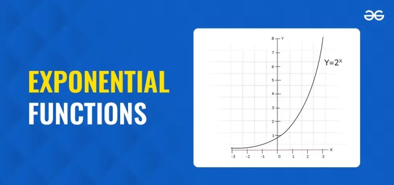
Graphically, the exponential function formula produces a curve that starts shallow but steepens rapidly, illustrating how small changes in \( x \) lead to massive changes in \( f(x) \) as \( x \) increases. This property is why exponential functions are used to model phenomena like Moore’s Law (technology doubling) or the spread of diseases (where each infected person can infect multiple others). The formula’s symmetry—whether modeling growth or decay—makes it a universal tool for analyzing dynamic systems. For instance, in pharmacokinetics, the decay of a drug in the bloodstream follows \( f(t) = D \cdot e^{-kt} \), where \( D \) is the initial dose and \( k \) is the elimination rate. Here, the exponential function formula quantifies how the body processes substances over time.
Key Benefits and Crucial Impact
The exponential function formula isn’t just a mathematical curiosity—it’s a framework for understanding systems where feedback loops amplify outcomes. In finance, it explains why reinvesting dividends can turn modest savings into fortunes over decades. In biology, it describes how a single mutation can spread through a population if it confers a survival advantage. Even in social media, the formula governs how a single viral post can reach millions in hours. Its impact is most pronounced in fields where small initial advantages compound into dominance, such as competitive markets or evolutionary biology. The formula’s predictive power lies in its ability to extrapolate long-term trends from short-term data, making it indispensable for strategic planning.
Beyond prediction, the exponential function formula enables optimization. For example, in logistics, minimizing delivery times often follows an exponential decay curve, where small delays early in the process can cascade into massive inefficiencies. Similarly, in renewable energy, the cost of solar panels has followed an exponential decline, reducing barriers to adoption. The formula’s versatility stems from its ability to model both deterministic and probabilistic systems, whether calculating the half-life of a chemical or the expected time for a stock to double. Its applications are limited only by the imagination of the analyst.
— "Exponential functions are the mathematics of the universe’s hidden accelerators. They reveal how small, consistent actions can outpace even the most ambitious linear projections."
— Dr. Steven Strogatz, Mathematician and Author of The Joy of x
Major Advantages
- Scalability: The exponential function formula models unbounded growth, making it ideal for long-term projections where linear models fail (e.g., technology adoption, population growth).
- Feedback Loop Capture: It naturally represents systems where outputs reinforce inputs (e.g., compound interest, viral marketing), unlike linear models that assume constant rates.
- Differentiability: Exponential functions are smooth and continuous, enabling precise calculus-based analysis in physics and engineering.
- Empirical Validation: From radioactive decay to bacterial growth, the formula’s predictions align with observable phenomena, earning it trust across scientific disciplines.
- Algorithm Efficiency: In computer science, exponential-time algorithms (e.g., brute-force search) highlight the trade-offs between accuracy and computational cost, guiding optimization strategies.
Comparative Analysis
| Aspect | Exponential Function Formula | Linear Function |
|---|---|---|
| Growth Pattern | Multiplicative (e.g., \( 2^x \)) | Additive (e.g., \( mx + b \)) |
| Long-Term Behavior | Unbounded (e.g., \( e^x \) → ∞ as \( x \) → ∞) | Bounded by slope (e.g., \( y = 2x \) grows linearly) |
| Applications | Compound interest, population growth, viral spread | Simple interest, linear depreciation, budgeting |
| Mathematical Tools | Logarithms, calculus (derivatives/integrals) | Basic arithmetic, slope-intercept form |
Future Trends and Innovations
The exponential function formula will continue to evolve alongside data science and AI. As machine learning models grow more complex, exponential functions will play a pivotal role in training curves, where loss functions often exhibit exponential decay. In quantum computing, exponential speedups (e.g., Shor’s algorithm) promise to revolutionize cryptography and optimization. Meanwhile, climate science will rely on exponential models to project tipping points in ecosystems, where small changes in temperature can trigger cascading effects. The formula’s future may also intersect with biology, as researchers use it to model epigenetic inheritance or the spread of antibiotic resistance.
One emerging trend is the hybridization of exponential functions with other mathematical frameworks. For example, logistic growth models (which combine exponential and linear terms) are increasingly used to predict saturation points in markets or resource depletion. Similarly, stochastic exponential models (incorporating randomness) are improving financial risk assessments. As computational power expands, the formula’s applications will extend to real-time systems, such as autonomous vehicles adapting to exponential response times or smart grids optimizing energy distribution. The next decade may even see exponential functions integrated into neuromorphic computing, mimicking the brain’s own recursive feedback loops.

Conclusion
The exponential function formula is more than a tool—it’s a lens through which we understand acceleration in nature and human systems. Its power lies in its simplicity: a constant ratio applied iteratively can reshape entire industries, ecosystems, or economies. Whether you’re analyzing the spread of an innovation, the decay of a radioactive isotope, or the growth of a portfolio, the formula provides a framework to anticipate outcomes that linear thinking cannot. The key to harnessing it is recognizing where multiplicative processes dominate, then applying the right parameters to the equation.
As fields like AI, biotech, and climate science push boundaries, the exponential function formula will remain central to innovation. Its ability to model both growth and decay ensures its relevance across disciplines, from the microscopic (quantum tunneling) to the macroscopic (galactic expansion). For professionals and students alike, mastering this formula isn’t just about solving equations—it’s about gaining a deeper intuition for how the world accelerates, decays, and transforms over time.
Comprehensive FAQs
Q: How is the exponential function formula different from a power function?
A: The exponential function formula (e.g., \( a \cdot b^x \)) has the variable in the exponent, while a power function (e.g., \( a \cdot x^b \)) has the variable as the base. This distinction means exponential functions grow/decay at rates proportional to their current value, whereas power functions grow at rates proportional to \( x \). For example, \( 2^x \) grows exponentially, but \( x^2 \) grows polynomially.
Q: Can the exponential function formula model negative growth?
A: Yes. When the base \( b \) is between 0 and 1 (e.g., \( 0.5 \)), the function decays exponentially, representing negative growth. This is common in half-life calculations (e.g., \( f(t) = a \cdot (0.5)^{t/T} \), where \( T \) is the half-life period). The formula can also model oscillatory behavior if combined with trigonometric terms.
Q: Why is \( e \) (Euler’s number) special in the exponential function formula?
A: \( e \) is the base of the natural exponential function (\( e^x \)) because it’s the limit of \( (1 + \frac{1}{n})^n \) as \( n \) approaches infinity, making it the most efficient base for continuous growth. Its derivative and integral are identical (\( \frac{d}{dx} e^x = e^x \)), simplifying calculus operations. Many natural processes (e.g., radioactive decay, bacterial growth) align closely with \( e^x \) due to its inherent connection to continuous compounding.
Q: How do I solve an exponential equation like \( 3 \cdot 2^x = 24 \)?
A: Divide both sides by 3 to isolate the exponential term: \( 2^x = 8 \). Recognize that \( 8 = 2^3 \), so \( x = 3 \). For more complex equations (e.g., \( 5 \cdot e^{2x} = 10 \)), take the natural logarithm of both sides: \( \ln(5 \cdot e^{2x}) = \ln(10) \), then solve for \( x \) using logarithm properties (\( \ln(a \cdot b) = \ln(a) + \ln(b) \)).
Q: What are common mistakes when applying the exponential function formula?
A:
- Misidentifying the base: Confusing \( b \) (e.g., 2 in \( 2^x \)) with the exponent. For example, \( 3^x \) grows faster than \( 2^x \) because the base is larger.
- Ignoring initial conditions: Forgetting the coefficient \( a \) (e.g., \( f(x) = 5 \cdot 2^x \) starts at 5, not 1).
- Linear vs. exponential confusion: Assuming \( 2^x \) grows as \( 2x \). Always check whether the variable is in the base or exponent.
- Incorrect logarithm application: Forgetting to divide exponents when taking logs (e.g., \( \ln(2^{3x}) = 3x \ln(2) \), not \( x \ln(2) \)).
- Overlooking units: In real-world problems, ensure \( x \) and \( b \) are dimensionally consistent (e.g., \( b \) might be a percentage converted to decimal).
Q: Where can I find real-world datasets to practice the exponential function formula?
A: Public repositories like Kaggle, Data.world, and government databases (e.g., U.S. Census) offer datasets on population growth, stock prices, and scientific measurements. For finance, platforms like Yahoo Finance provide historical returns to model compound interest. Start with simple time-series data (e.g., daily temperatures) to fit exponential curves using tools like Python’s `scipy.optimize.curve_fit`.
Leave a Comment
Comments are moderated before appearing. The data you submit is processed according to the Privacy Policy of Bevvy.