How the k-means algorithm reshapes data science and machine learning
The k-means algorithm isn’t just another tool in the data scientist’s arsenal—it’s a foundational pillar of unsupervised learning, quietly powering everything from customer segmentation to image compression. Its simplicity belies its versatility: a method that distills complex datasets into meaningful clusters with minimal computational overhead. Yet for all its ubiquity, the algorithm’s core mechanics—how it balances centroid initialization, iterative optimization, and convergence criteria—remain misunderstood by even seasoned practitioners. The result? Missed opportunities in precision, scalability, and interpretability.
What makes the k-means algorithm tick isn’t just its mathematical elegance but its adaptability. Whether applied to high-dimensional genomic data or low-latency recommendation systems, it thrives where labels are absent and patterns must be inferred. The challenge lies in mastering its nuances: the trade-offs between Euclidean distance metrics and Manhattan alternatives, the pitfalls of poor centroid seeding, and the subtle art of determining the optimal k. These decisions can mean the difference between actionable insights and statistical noise.
Critics often dismiss the k-means algorithm as outdated, overshadowed by deep learning’s hype. But its resilience stems from a counterintuitive truth: sometimes, the most effective solutions are the simplest. While neural networks demand vast data and computational power, the k-means algorithm delivers interpretable, scalable results with minimal prerequisites. Its enduring relevance lies in its ability to serve as both a standalone solution and a preprocessing step—bridging the gap between raw data and sophisticated models.
The Complete Overview of the k-means Algorithm
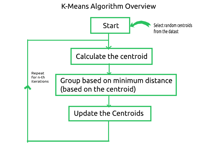
The k-means algorithm is a cornerstone of unsupervised learning, designed to partition a dataset into k distinct, non-overlapping clusters based on feature similarity. Unlike supervised methods that rely on labeled data, this clustering technique excels in exploratory analysis, where the goal is to uncover hidden structures without predefined categories. Its appeal lies in its balance of efficiency and interpretability: by minimizing within-cluster variance (typically measured via Euclidean distance), the algorithm iteratively refines cluster assignments until convergence. This iterative process—assigning data points to the nearest centroid, then recalculating centroids—forms the backbone of its functionality.
Yet its simplicity masks critical design choices. The selection of k isn’t arbitrary; it’s a hyperparameter that demands domain knowledge. Too few clusters risk oversimplification, while too many may reveal spurious patterns. Similarly, the initialization of centroids—whether via random sampling, k-means++ for smarter seeding, or deterministic methods—directly impacts convergence speed and final cluster quality. These factors explain why the k-means algorithm, despite its age, remains a dynamic field of research, with ongoing refinements in initialization strategies, distance metrics, and parallelization techniques.
Historical Background and Evolution
The k-means algorithm traces its origins to 1957, when Stuart Lloyd of Bell Labs formalized its iterative optimization framework for pulse-code modulation in telecommunications. However, its theoretical underpinnings were independently rediscovered in the 1960s by statisticians and computer scientists, cementing its place in clustering literature. The algorithm’s early adoption in pattern recognition and image segmentation highlighted its utility in domains where human annotation was impractical. By the 1980s, its integration into statistical software like R and MATLAB democratized access, making it a staple in academic and industrial workflows.
Table of Contents
- The Complete Overview of the k-means Algorithm
- Historical Background and Evolution
- Core Mechanisms: How It Works
- Key Benefits and Crucial Impact
- Major Advantages
- Comparative Analysis
- Future Trends and Innovations
- Conclusion
- Comprehensive FAQs
- Q: How do I choose the optimal number of clusters ( k ) for the k-means algorithm?
- Q: Why does the k-means algorithm sometimes produce empty clusters?
- Q: Can the k-means algorithm handle non-numeric data (e.g., text or categorical variables)?
- Q: How does the k-means algorithm perform with high-dimensional data?
- Q: What are the main limitations of the k-means algorithm, and when should I avoid it?
Evolutionary milestones include the introduction of k-means++ in 2007, which mitigated the sensitivity to initial centroid placement by probabilistically selecting seeds based on data density. Subsequent advancements—such as spherical k-means for high-dimensional data and fuzzy k-means for probabilistic assignments—expanded its applicability. Today, variants like Mini-Batch k-means and its GPU-accelerated counterparts address scalability challenges in big data environments, proving that the algorithm’s core principles remain adaptable to modern computational constraints.
Core Mechanisms: How It Works
At its core, the k-means algorithm operates on two alternating steps: assignment and update. In the assignment phase, each data point is allocated to the nearest centroid using a chosen distance metric (most commonly Euclidean). The update phase then recalculates centroids as the mean of all points assigned to their respective clusters. This cycle repeats until centroids stabilize or a maximum iteration limit is reached. The algorithm’s efficiency stems from its use of squared Euclidean distances, which avoids costly square root operations while preserving optimality under certain conditions.
Convergence is guaranteed under specific assumptions—namely, that the dataset is spherical and clusters are of similar size—but real-world data rarely meets these criteria. This is where variants like k-medoids (using medians instead of means) or hierarchical clustering come into play. The choice of distance metric further complicates the landscape: while Euclidean distance dominates, cosine similarity or Manhattan distance may better suit sparse or high-dimensional data. Understanding these trade-offs is essential for deploying the k-means algorithm effectively in practice.
Key Benefits and Crucial Impact
The k-means algorithm’s impact spans industries, from retail (customer segmentation) to genomics (gene expression clustering). Its ability to handle large datasets with minimal computational overhead makes it ideal for preprocessing tasks, such as reducing dimensionality before applying more complex models. In natural language processing, it’s used for topic modeling and document clustering, while in computer vision, it segments images and detects anomalies. The algorithm’s scalability—especially in distributed computing frameworks like Apache Spark—further amplifies its reach.
Beyond technical advantages, the k-means algorithm offers interpretability. Clusters can be visualized, labeled, and validated using metrics like the silhouette score or Davies-Bouldin index, providing tangible insights into data structure. This transparency contrasts sharply with black-box models, where feature importance is opaque. For businesses, the algorithm’s ability to group customers, products, or transactions into actionable segments translates directly into revenue growth and operational efficiency.
— "The k-means algorithm is not just a tool; it’s a lens that reveals the inherent geometry of data. Its simplicity is its superpower."
— Dr. David Donoho, Stanford University (Statistical Learning Theory)
Major Advantages
- Computational Efficiency: Linear time complexity relative to dataset size (O(n) per iteration), making it suitable for large-scale applications.
- Scalability: Parallelizable variants (e.g., Mini-Batch k-means) leverage distributed computing for real-time processing.
- Interpretability: Clusters are geometrically intuitive, with centroids serving as prototypical representatives.
- Versatility: Adaptable to diverse distance metrics (Euclidean, Manhattan, cosine) and data types (numeric, text, images).
- Foundation for Advanced Models: Often used as a preprocessing step for deep learning (e.g., autoencoders) or as a baseline for comparison.

Comparative Analysis
| k-means Algorithm | Hierarchical Clustering |
|---|---|
|
|
| DBSCAN | Gaussian Mixture Models (GMM) |
|
|
Future Trends and Innovations
The k-means algorithm’s future lies in hybrid approaches that marry its efficiency with modern techniques. For instance, integrating it with deep learning—such as using k-means for prototype selection in neural networks—could reduce training data requirements while preserving interpretability. Advances in quantum computing may also redefine its scalability, enabling clustering of exponentially larger datasets. Meanwhile, research into adaptive k-selection (via information criteria or Bayesian nonparametrics) aims to automate one of its most critical hyperparameters.
Another frontier is explainable AI, where the k-means algorithm’s clusters serve as feature explanations for black-box models. By decomposing complex predictions into interpretable segments, it bridges the gap between performance and transparency. As data grows more heterogeneous—combining text, images, and time-series—variants like multi-view k-means or deep embedding clustering will likely dominate. The algorithm’s legacy, then, isn’t stagnation but continuous reinvention.

Conclusion
The k-means algorithm endures because it solves a fundamental problem: how to organize chaos into meaningful order. Its strength isn’t in being the most sophisticated tool but in being the most accessible—democratic in its application and robust in its results. For practitioners, the key lies in recognizing its limitations (e.g., sensitivity to outliers, assumption of convex clusters) and pairing it with complementary methods. Whether used for exploratory data analysis or as a preprocessing step, its role in the machine learning pipeline remains indispensable.
As data science evolves, the k-means algorithm will continue to adapt, proving that sometimes, the most powerful solutions are those built on decades of refinement rather than fleeting trends. Its story is a testament to the enduring value of mathematical rigor and practical ingenuity—a reminder that in an era of complexity, simplicity often holds the key.
Comprehensive FAQs
Q: How do I choose the optimal number of clusters (k) for the k-means algorithm?
A: The optimal k is typically determined using the elbow method (plotting within-cluster sum of squares vs. k and selecting the "elbow" point) or metrics like the silhouette score (measuring cluster cohesion/separation). Domain knowledge also plays a role—e.g., if you’re segmenting customers, k might align with business strategies (e.g., 3 tiers: high, medium, low value).
Q: Why does the k-means algorithm sometimes produce empty clusters?
A: Empty clusters occur when centroids are initialized in sparse regions of the data, causing all points to be assigned to other clusters. This is mitigated by k-means++ initialization, which spreads centroids based on data density, or by using k-medoids (where centroids are actual data points). Preprocessing (e.g., scaling features) can also reduce this issue.
Q: Can the k-means algorithm handle non-numeric data (e.g., text or categorical variables)?
A: The standard k-means algorithm requires numeric inputs, but it can be adapted for text via TF-IDF or word embeddings (e.g., converting documents to vectors) or for categorical data by encoding variables (e.g., one-hot encoding) or using distance metrics like Gower’s distance. For mixed data, techniques like multiple correspondence analysis (MCA) may be needed.
Q: How does the k-means algorithm perform with high-dimensional data?
A: In high dimensions, Euclidean distance becomes less meaningful due to the "curse of dimensionality" (all points appear equidistant). Solutions include:
- Using PCA or t-SNE for dimensionality reduction before clustering.
- Switching to cosine similarity or Manhattan distance.
- Employing spherical k-means, which normalizes data to unit vectors.
Q: What are the main limitations of the k-means algorithm, and when should I avoid it?
A: Avoid the k-means algorithm when:
- Clusters are non-spherical or varying in density (use DBSCAN or GMM instead).
- Data contains outliers or noise (k-medoids or robust variants may help).
- You need probabilistic assignments (GMM provides soft clustering).
- The dataset is very large and sparse (consider approximate methods like Mini-Batch k-means).
- Clusters are hierarchical or overlapping (hierarchical clustering or spectral clustering is better).
Leave a Comment
Comments are moderated before appearing. The data you submit is processed according to the Privacy Policy of Bevvy.